Create semi-additive measures

In general, there are three kinds of measures:

• Additive These measures are aggregated by using the SUM function across any dimensions. A typical example is revenue, which can be added across different product categories, cities, and dates, as well as other dimensions. Revenue of all months within a year, when added together, equals the total year revenue.
• Semi-additive These measures can be added across some but not all dimensions. For example, inventory counts can be added across different product categories and cities, but not dates; if you had five units yesterday and two units today, that doesn’t mean you’ll have seven units tomorrow. On the other hand, if you have five units in Sydney and two units in Melbourne, this means you’ve got seven units in the two cities in total.
• Non-additive These measures cannot be added across any dimensions. For instance, you cannot add up the average price across any dimension, because the result would not make any practical sense. If the average sale price in Sydney was $4.50, and it was $3.50 in Melbourne, you cannot say that across both cities, the average price was $8.00 or even $4.00 because the number of units sold could be very different.

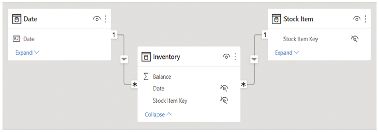
In this section, we focus on semi-additive measures. There are several ways to write a semi-additive measure, and the correct way for you depends on your business requirements. Let’s say your business is interested in inventory counts, and you have the data model shown in Figure 2-27.

FIGURE 2-27 Inventory data model

If you have inventory figures for all dates of interest in your data, you can write the following measure:

Inventory Balance =
CALCULATE(
    SUM(Inventory[Balance]),
    LASTDATE(‘Date'[Date])
)

In addition to LASTDATE and its sister function FIRSTDATE, there are some DAX functions that can help you retrieve the opening or closing balance for different time periods:

• OPENINGBALANCEMONTH
• OPENINGBALANCEQUARTER
• OPENINGBALANCEYEAR
• CLOSINGBALANCEMONTH
• CLOSINGBALANCEQUARTER
• CLOSINGBALANCEYEAR

The functions that start with CLOSING evaluate an expression for the last date in the period, and the functions that start with OPENING evaluate an expression for one day before the first date in the period. This means that the opening balance for February 1 is the same as the closing balance for January 31.

For example, you can calculate the opening month balance for inventory as follows:

Click here to view code image

Inventory Opening Balance Month =
OPENINGBALANCEMONTH(
    SUM(Inventory[Balance]),
    ‘Date'[Date]
)

The date-based functions listed here only work if you have data for all dates of interest. For example, if you’d chosen to use CLOSINGBALANCEMONTH but your data ends on May 23, 2022, as is the case for sample data, you’d get a blank value for May 2022. For cases such as this, you can use LASTNONBLANKVALUE or FIRSTNONBLANKVALUE as shown here:

Inventory Last Nonblank =
LASTNONBLANKVALUE(
    ‘Date'[Date],
    SUM(Inventory[Balance])
)

This measure will show the latest available balance in the current context.

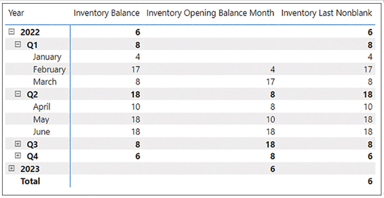
The Inventory Balance, Inventory Opening Balance Month, and Inventory Last Nonblank measures can be seen in Figure 2-28.

FIGURE 2-28 Inventory measures

Determining which calculation you should use depends on your business requirements—there is no single correct answer that applies to all scenarios. Missing data may mean there’s no inventory, or it may mean that data isn’t captured frequently enough, so the data modeler should understand the underlying data before writing the calculations to ensure the data isn’t represented incorrectly.